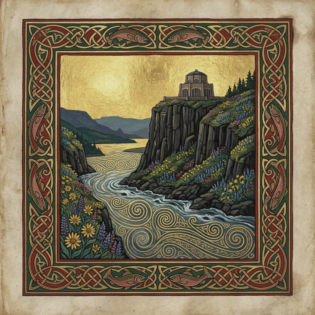
Navigating Remote Expeditions: 3D Google Earth Photogrammetry & VRP Routing

The Landscape Photographer’s Dilemma: Time, Light, and Distance

Every landscape and expedition photographer understands the cruelty of natural light. The most magical photographic windows—astronomical twilight, blue hour, and the flaming hues of golden hour—last only 20 to 45 minutes twice a day. Meanwhile, the physical landscape is immense, rugged, and indifferent to our schedules.

When planning multi-day field expeditions across thousands of square miles (such as navigating Oregon’s 36 counties or traversing the Pacific Rim Highway 101), traditional road trip planning falls apart. Estimating drive times with standard GPS navigation ignores:

1. Strict Sun and Solar Azimuth Windows: Arriving 15 minutes late means missing the fleeting sidelight on an alpine ridge.
2. Topographic Horizon Occlusion: A 10,000-foot volcanic summit blocks direct sunlight long before astronomical sea-level sunset.
3. Setup and Hike Slack Time: Parking, packing 35 lbs of optical gear, hiking a 1,200-foot ascent, and leveling a tripod takes predictable, non-zero time.
4. Energy and Backcountry Range Constraints: Fuel stops, EV charging curves, and driver fatigue limits.

To solve this, I transformed my field expedition workflows into a two-stage computational system: 3D Virtual Terrain Scouting in Google Earth coupled with Vehicle Routing Problems with Time Windows (VRPTW) solved in Google Colab.

Phase 1: Virtual Photogrammetry & Line-of-Sight in Google Earth

Before writing a single line of code or packing a camera bag, every prospective waypoint undergoes line-of-sight and topographic analysis in Google Earth.

1. 3D Terrain & Focal Angle Modeling

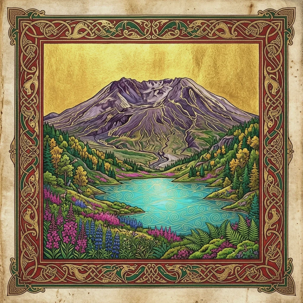
By enabling Google Earth’s photorealistic 3D terrain mesh, you can position the virtual camera at ground level (e.g., 5.5 feet above terrain) at the exact coordinates of your prospective tripod placement.

• Field-of-View (FOV) Emulation: Adjusting Google Earth’s camera field of view allows you to simulate whether a 16mm ultra-wide or an 85mm telephoto is required to frame the mountain peak within the canyon walls.
• Sun & Shadow Animation: Google Earth’s sunlight slider allows you to scrub through the exact day of the year to observe how mountain ridges cast shadows across valleys and lakes.

2. Waypoint Metadata Extraction

Once vantage points and trailheads are locked in, export them as a structured GeoJSON or KML file containing:

• Landmark name & County
• Precise Lat/Lng coordinates
• Elevation in feet
• Target Sun Altitude & Azimuth
• Minimum Setup & Tear-down duration (e.g., 45 minutes)

Phase 2: Formulating the Photographer’s Vehicle Routing Problem (VRPTW)

In operations research, the Vehicle Routing Problem with Time Windows (VRPTW) is a generalization of the classic Traveling Salesperson Problem (TSP).

Instead of merely finding the shortest loop connecting a list of cities, VRPTW incorporates:

• Time Windows $[e_i, l_i]$: Earliest arrival time $e_i$ and latest departure time $l_i$ for waypoint $i$. For sunrise photography, this window is tightly bounded to $[T_{dawn} - 30\text{m}, T_{sunrise} + 20\text{m}]$.
• Service Duration $s_i$: The time spent on-site shooting brackets, scouting compositions, and repacking.
• Transit Duration Matrix $D_{ij}$: The actual driving and hiking transit time between location $i$ and location $j$.

[Base Camp / Hub] ──(Transit)──> [Dawn Scout: Coastal Bluff]
                                       │
                              (Golden Hour Window: 06:15 - 06:55)
                                       │
                                   (Transit)
                                       ↓
                             [Midday: Dense Rainforest]
                                       │
                              (High Overcast Canopy: 11:30 - 13:30)
                                       │
                                   (Transit)
                                       ↓
                             [Dusk: High Desert Butte]
                                       │
                              (Sunset Window: 18:40 - 19:25)
                                       ↓
                             [Night Base Camp / Hotel]

Phase 3: The Google Colab Optimization Pipeline

Using Google Colab and Google’s open-source OR-Tools suite, we can rapidly generate the optimal multi-day expedition itinerary.

1. Setting Up Google OR-Tools in Colab

In your Colab notebook, install the routing libraries:

!pip install -q ortools geopandas shapely requests

2. Distance Matrix Calculation

We build a symmetric or asymmetric duration matrix using OpenStreetMap routing (OSRM) or the Google Routes API:

import numpy as np
from ortools.constraint_solver import routing_enums_pb2
from ortools.constraint_solver import pywrapcp

# Define Waypoints: (Name, Earliest Min, Latest Min, Service Duration Min)
# Time expressed in minutes from 00:00 (e.g., 06:00 AM = 360 min)
WAYPOINTS = [
    {"name": "Base Camp (Portland)", "window": (0, 1440), "service": 0},
    {"name": "Peter Iredale Shipwreck", "window": (375, 435), "service": 50}, # Sunrise
    {"name": "Ecola State Park Bluff", "window": (510, 600), "service": 40},
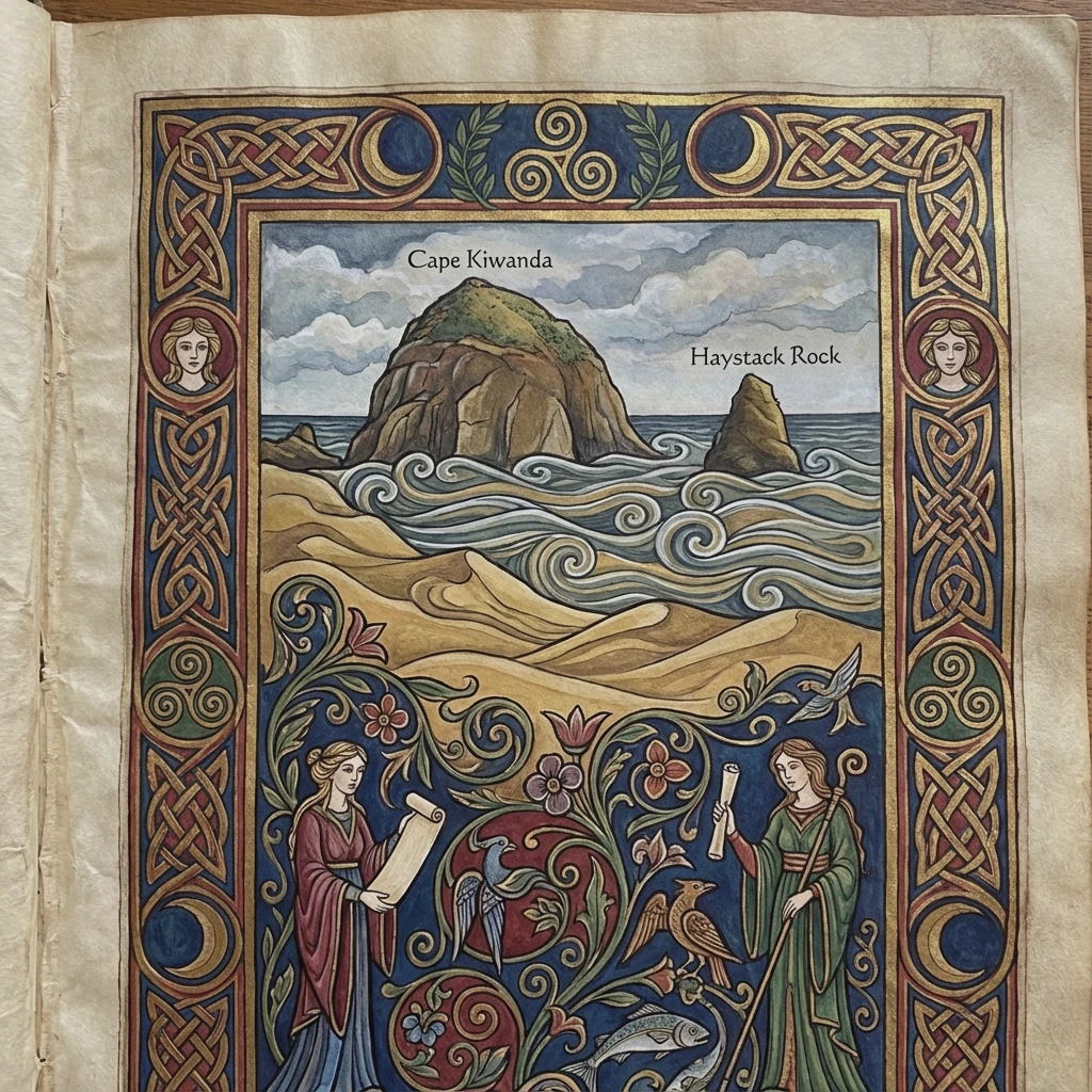
    {"name": "Cape Kiwanda Dory Launch", "window": (1080, 1170), "service": 60}, # Sunset
    {"name": "Timberline Lodge", "window": (1200, 1320), "service": 45}, # Blue Hour / Night
]

# Transit duration matrix in minutes (simulated example)
transit_matrix = [
    [0, 110, 95, 120, 75],
    [110, 0, 35, 85, 160],
    [95, 35, 0, 70, 145],
    [120, 85, 70, 0, 140],
    [75, 160, 145, 140, 0]
]

3. Solver Configuration with Time Windows

def solve_photo_expedition():
    manager = pywrapcp.RoutingIndexManager(len(transit_matrix), 1, 0)
    routing = pywrapcp.RoutingModel(manager)

    def time_callback(from_index, to_index):
        from_node = manager.IndexToNode(from_index)
        to_node = manager.IndexToNode(to_index)
        return transit_matrix[from_node][to_node] + WAYPOINTS[from_node]["service"]

    transit_callback_index = routing.RegisterTransitCallback(time_callback)
    routing.SetArcCostEvaluatorOfAllVehicles(transit_callback_index)

    # Add Time Dimension with Max 24-Hour Horizon (1440 minutes)
    time_dimension_name = 'Time'
    routing.AddDimension(
        transit_callback_index,
        60,    # Max waiting/slack time allowed
        1440,  # Max total trip time
        False, # Don't force start cumul to zero
        time_dimension_name
    )
    time_dimension = routing.GetDimensionOrDie(time_dimension_name)

    # Set Time Windows for each waypoint
    for node, wp in enumerate(WAYPOINTS):
        index = manager.NodeToIndex(node)
        time_dimension.CumulVar(index).SetRange(wp["window"][0], wp["window"][1])

    # Search parameters
    search_parameters = pywrapcp.DefaultRoutingSearchParameters()
    search_parameters.first_solution_strategy = (
        routing_enums_pb2.FirstSolutionStrategy.PATH_CHEAPEST_ARC
    )

    solution = routing.SolveWithParameters(search_parameters)
    return manager, routing, solution

Field Telemetry Example: The Pacific Edge Capture

Here is the exact camera telemetry captured at the termination of an algorithmic run at the Shipwreck of the Peter Iredale during astronomical low-tide sunset:

Phase 4: Adaptive Re-Routing in the Field

No plan survives first contact with coastal fog or sudden mountain pass closures.

Because the entire routing pipeline resides in a lightweight Google Colab notebook, I can pull up the notebook on a mobile device or tablet from a trailhead:

1. Flag a waypoint as closed or weather_compromised.
2. Re-execute the cell with updated current GPS coordinates as the new origin.
3. Obtain a brand-new, globally optimal sequence within 1.8 seconds.

Conclusion: Engineering the Perfect Shot

Great landscape photography will always demand patience, artistic intuition, and an eye for emotional resonance. But removing logistical friction through Google Earth photogrammetry and OR-Tools optimization ensures that when the sky turns crimson, you aren’t stuck in traffic thirty miles away—you are standing on the precipice with your tripod locked, ready for the light.